How to Find Records with the Data Form in Excel 20130

In a large data list, trying to find a particular record by moving from record to record in Excel 2013 — or even moving ten records at a time with the scroll bar — can take all day. Rather than waste time trying to manually search for a record, you can use the Criteria button in the data form to look it up.

When you click the Criteria button, Excel clears all the field entries in the data form (and replaces the record number with the word Criteria) so that you can enter the criteria to search for in the blank text boxes.

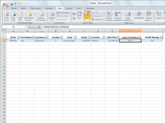
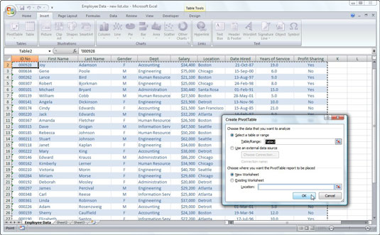
For example, suppose that you need to edit Sherry Caulfield’s profit sharing status. Unfortunately, her paperwork doesn’t include her ID number. All you know is that she works in the Boston office and spells her last name with a C instead of a K.

To find her record, you can use the information you have to narrow the search to all the records where the last name begins with the letter C and the Location field contains Boston.

To limit your search in this way, open the data form for the Employee Data database, click the Criteria button, and then type C* in the text box for the Last Name field. Also enter Boston in the text box for the Location field.

When you enter search criteria for records in the blank text boxes of the data form, you can use the ? (for single) and * (for multiple) wild-card characters.

Now click the Find Next button. Excel displays in the data form the first record in the database where the last name begins with the letter C and the Location field contains Boston. The first record in this data list that meets these criteria is for William Cobb. To find Sherry’s record, click the Find Next button again. Sherry Caulfield’s record then shows up.

Having located Caulfield’s record, you can then edit her profit sharing status from No to Yes in the text box for the Profit Sharing field. When you click the Close button, Excel records her new profit sharing status in the data list.

When you use the Criteria button in the data form to find records, you can include the following operators in the search criteria you enter to locate a specific record in the database:

Operator	Meaning
=	Equal to
>	Greater than
>=	Greater than or equal to
<	Less than
<=	Less than or equal to
<>	Not equal to

For example, to display only those records where an employee’s salary is greater than or equal to $50,000, enter >=50000 in the text box for the Salary field and then click the Find Next button.

When specifying search criteria that fit a number of records, you may have to click the Find Next or Find Prev button several times to locate the record you want. If no record fits the search criteria you enter, the computer beeps at you when you click these buttons.

To change the search criteria, first clear the data form by clicking the Criteria button again and then clicking the Clear button.

To switch back to the current record without using the search criteria you enter, click the Form button. (This button replaces the Criteria button as soon as you click the Criteria button.)

Read More...

How to Name a Cell or Cell Range in Excel 20130

By assigning descriptive names to cells and cell ranges in Excel 2013, you can go a long way toward keeping on top of the location of important information in a worksheet. Rather than try to associate random cell coordinates with specific information, you just have to remember a name.

You can also use range names to designate the cell selection that you want to print or use in other Office 2013 programs, such as Microsoft Word or Access. Best of all, after you name a cell or cell range, you can use this name with the Go To feature to not only locate the range but select all its cells as well.

When assigning range names to a cell or cell range, you need to follow a few guidelines:

• Range names must begin with a letter of the alphabet, not a number.
  For example, instead of 01Profit, use Profit01.
• Range names cannot contain spaces.
  Instead of a space, use the underscore (Shift+hyphen) to tie the parts of the name together. For example, instead of Profit 01, use Profit_01.
• Range names cannot correspond to cell coordinates in the worksheet.
  For example, you can’t name a cell Q1 because this is a valid cell coordinate. Instead, use something like Q1_sales.

To name a cell or cell range in a worksheet, follow these steps:

1. Select the cell or cell range that you want to name.
2. Click the cell address for the current cell that appears in the Name Box on the far left of theFormula bar.
   Excel selects the cell address in the Name Box.
3. Type the name for the selected cell or cell range in the Name Box.
   When typing the range name, you must follow Excel’s naming conventions.
4. Press Enter.

To select a named cell or range in a worksheet, click the range name on the Name Box drop-down list. To open this list, click the drop-down arrow button that appears to the right of the cell address on the Formula bar.

You can also accomplish the same thing by selecting Home→Find & Select→Go To or by pressing F5 or Ctrl+G to open the Go To dialog box. Double-click the desired range name in the Go To list box. Excel moves the cell cursor directly to the named cell. If you select a cell range, all the cells in that range are selected as well.

Read More...

How to Create a Table in Excel 20070

You can create a table in Excel 2007 (a list or database in previous Excel versions) to help you manage and analyze related data. The purpose of an Excel table is not so much to calculate new values but rather to store lots of information in a consistent manner, making it easier to format, sort, and filter worksheet data. Typically, an Excel table has only column headings and no row headings.

An Excel table is not the same as a data table that can be used for what-if analysis. You use a data table to show how changing one or two variables in formulas affects the results of those formulas.

1

Enter your table's column headings.

Click the blank cell where you want to start the new table and then enter the column headings (such as ID No, First Name, Last Name, Dept, and so on) in separate cells within the same row. Column headings are also known asfield names. The column headings should appear in a single row without any blank cells between the entries.

2

Enter the first row of data immediately below the column headings you typed in Step 1.

These entries constitute the first row, or record, of the table.

3

Click the Table command button in the Tables group of the Insert tab.

Excel displays a marquee around all the cells in the new table. The Create Table dialog box appears, listing the address of the table in the Where Is the Data for Your Table text box. (If the address displayed here is incorrect, drag in the worksheet to select the correct range.)

4

Click the My Table Has Headers check box to select it.

These headers are the column headings entered in the first step.

 Enlarge

5

Click OK.

Excel inserts and formats the new table and adds filter arrows (drop-down buttons) to each of the field names in the top row.

Another way to insert a table is to click the Format as Table button in the Styles group on the Home tab and then select a table style of your choice in the gallery that appears. Use this method if you want to apply a different table style as you create a table.

If you want to convert an existing Excel table back to a normal range of cells, select any cell in the table and then click the Convert to Range button on the Table Tools Design tab. All data and formatting is preserved.

Read More...

How to Repeat Row and Column Headings When You Print in Excel 20070

Excel 2007’s Print Titles command enables you to print particular row and column headings on each page of the report. Print titles are important in multipage reports where the columns and rows of related data spill over to other pages that no longer show the row and column headings.

Don’t confuse print titles with the header of a report. Even though both are printed on each page, header information prints in the top margin of the report; print titles always appear in the body of the report — at the top, in the case of rows used as print titles, and on the left, in the case of columns.

1

Click the Print Titles button on the Ribbon’s Page Layout tab.

The Page Setup dialog box appears with the Sheet tab selected.

 Enlarge

2

To designate worksheet rows as print titles, select the Rows to Repeat at Top text box and then drag through the row number(s) (in the worksheet frame) with data you want to appear at the top of each page.

If necessary, reduce the Page Setup dialog box to just the Rows to Repeat at Top text box by clicking the text box’s Collapse/Expand button.

3

To designate worksheet columns as print titles, select the Columns to Repeat at Left text box and then drag through the column letter(s) (in the worksheet frame) with the data you want to appear at the left edge of each page.

If necessary, reduce the Page Setup dialog box to just the Columns to Repeat at Left text box by clicking its Collapse/Expand button.

 Enlarge

4

Click OK.

You can preview the worksheet to determine if the print titles are set up correctly.

To clear print titles from a report if you no longer need them, open the Sheet tab of the Page Setup dialog box and then delete the row and column ranges from the Rows to Repeat at Top and the Columns to Repeat at Left text boxes before you click OK.

Read More...

How to Protect an Excel 2007 Workbook0

Excel 2007 includes a Protect Workbook command that prevents others from making changes to the layout of the worksheets in a workbook. You can assign a password when you protect a workbook so that only those who know the password can unprotect the workbook and make changes to the structure and layout of the worksheets.

Protecting a workbook does not prevent others from making changes to the contents ofcells. To protect cell contents, you must use the Protect Sheet command button on the Review tab.

Protecting a workbook

Follow these steps to protect an Excel 2007 workbook:

1. Click the Protect Workbook command button in the Changes group on the Review tab.
   Excel opens the Protect Structure and Windows dialog box, where the Structure check box is selected by default. With the Structure check box selected, Excel won’t let anyone mess around with the sheets in the workbook (by deleting them or rearranging them).
   
   

   You can protect the structure and windows in a workbook.
2. (Optional) If you want to protect any windows that you set up, select the Windows check box.
   When selected, this setting keeps the workbook windows in the same size and position each time you open the workbook.
3. To assign a password that must be supplied before you can remove the protection from the worksheet, type the password in the Password (optional) text box.
4. Click OK.
   If you typed a password in the Password (optional) text box, Excel opens the Confirm Password dialog box. Re-enter the password in the Reenter Password to Proceed text box exactly as you typed it Step 3, and then click OK.

Unprotecting a workbook

To remove protection from the current workbook, follow these steps:

1. Click the Unprotect Workbook command button in the Changes group on the Review tab.
2. If you assigned a password when protecting the workbook, type the password in the Password text box and click OK.

Protecting a shared workbook

If you create a workbook with contents to be updated by several different users on your network, you can use the Protect and Share Workbook command to ensure that Excel tracks all the changes made and that no user can intentionally or inadvertently remove Excel’s tracking of changes. Follow these steps:

1. Click the Protect and Share Workbook command button in the Changes group on the Review tab.
   The Protect Shared Workbook dialog box appears.
2. Select the Sharing with Track Changes check box.
   
   

   Protect a shared workbook so that users cannot remove Excel’s tracking of changes.
3. To assign a password that each user must supply before he or she can open the workbook to make any changes, type a password in the Password (optional) text box and click OK.

Read More...

Using Logical Excel Functions in Excel 2007 Formulas0

Excel 2007 uses seven logical functions — AND, FALSE, IF, IFERROR, NOT, OR, and TRUE — which appear on the Logical command button’s drop-down menu on the Excel Formulas tab of the Ribbon. All the logical functions return either the logical TRUE or logical FALSE when their functions are evaluated.`

Here is an Excel functions list that shows the logical function with its argument syntax:

• AND(logical1,logical2,...) tests whether the logical arguments are TRUE or FALSE. If they are all TRUE, the AND function returns TRUE to the cell. If any are FALSE, the AND function returns FALSE.
• IF(logical_test,value_if_true,value_if_false) tests whether the logical_test expression is TRUE or FALSE. If TRUE, the Excel IF function returns the value_if_true argument. If FALSE, the IF function returns the value_if_false argument.
• IFERROR(value,value_if_error) tests whether the value expression is an error. IFERROR returnsvalue_if_error if the expression is an error, or value of the expression if it is not an error.
• NOT(logical) tests whether the logical argument is TRUE or FALSE. If TRUE, the NOT function returns FALSE. If FALSE, the NOT function returns TRUE.
• OR(logical1,logical2,...) tests whether the logical arguments are TRUE or FALSE. If any are TRUE, the OR function returns TRUE. If all are FALSE, the OR function returns FALSE.
• FALSE() — takes no argument and simply enters logical FALSE in its cell.
• TRUE() takes no argument and simply enters logical TRUE in its cell.

The logical_test and logical arguments that you specify for these logical functions usually employ the comparison operators (=, <, >, <=, >=, and <>), which themselves return logical TRUE or logical FALSE values. For example, suppose that you enter the following formula in your Excel worksheet:

=AND(B5=D10,C15>=500)

In this Excel formula, the spreadsheet program first evaluates the first logical argument to determine whether the contents in cell B5 and D10 are equal to each other. If they are, the first comparison returns TRUE. If they are not equal to each other, this comparison returns FALSE. The program then evaluates the second logical argument to determine whether the content of cell C15 is greater than or equal to 500. If it is, the second comparison returns TRUE. If it is not greater than or equal to 500, this comparison returns FALSE.

After evaluating the comparisons in the two logical arguments, the AND function compares the results: If logical argument 1 and logical argument 2 are both found to be TRUE, then the AND function returns logical TRUE to the cell. If, however, either argument is found to be FALSE, then the AND function returns FALSE to the cell.

When you use the IF function, you specify what’s called a logical_test argument whose outcome determines whether the value_if_true or value_if_false argument is evaluated and returned to the cell. The logical_test argument normally uses comparison operators, which return either the logical TRUE or logical FALSE value. When the argument returns TRUE, the entry or expression in the value_if_trueargument is used and returned to the cell. When the argument returns FALSE, the entry or expression in the value_if_false argument is used.

Consider the following formula that uses the Excel IF function to determine whether to charge tax on an item:

=IF(E5="Yes",D5+D5*7.5%,D5)

If cell E5 (the first cell in the column, where you indicate whether the item being sold is taxable or not) contains Yes, the IF function uses the value_if_true argument that tells Excel to add the extended price entered in cell D5, multiply it by a tax rate of 7.5%, and then add the computed tax to the extended price. If, however, cell D5 is blank or contains anything other than the text Yes, then the IF function uses the value_if_false argument, which tells Excel to just return the extended price in cell D5 without adding any tax to it.

As you can see, the value_if_true and value_if_false arguments of the Excel IF function can contain constants or expressions whose results are returned to the cell that holds the IF formula.

Read More...

How to Change Column Width and Row Height in Excel 20070

In Excel 2007, you can change any column widths or row heights in your worksheets to improve the readability and appearance of data. For example, if your worksheet contains many numbers, you can widen the columns to make the worksheet less cluttered. You should always widen columns that contain cells with truncated text entries or numbers that Excel shows as ######.

Based on the default 11-point Calibri font, the default column width is 8.43 and the default row height is 15. If you change the default font type or size, Excel may also change the standard column width or row height. You can manually set a default column width by choosing Format→Standard Width in the Cells group on the Home tab. You cannot manually set a default row height.

Adjusting column widths

Follow these steps to adjust the width of one or more columns:

1. Select the columns whose width you want to change.
   You select an entire column by clicking its column letter. If you want to adjust a single column, click any cell in that column.
2. Choose a method to adjust column width:
   • To manually change the width of columns, position the mouse pointer on the right boundary of a column heading until it turns into a double-sided arrow. Drag until the column is the width that you want.
     
     

     Drag a column boundary to manually change a column width.
   • To set a column width to a specific setting, choose Format→Column Width on the Home tab. Type the exact width you want in the Column Width dialog box; then click OK.
     
     

     Set a specific width in the Column Width dialog box.
   • To automatically change the column width so it fits the widest entry, use AutoFit. Double-click the boundary on the right side of the column heading or choose Format→AutoFit Column Width on the Home tab.

Changing row heights

To change the height of one or more rows, follow these steps:

1. Select the rows whose height you want to adjust.
   To select an entire row, click on the row number on the left. If you want to adjust a single row, click any cell in that row.
2. Choose a method to adjust row height:
   • To manually change the row height, position the mouse pointer on the bottom boundary of the row heading until it turns into a double-sided arrow. Drag until the row is the height that you want.
     
     

     Drag a row boundary to manually change the row height.
   • To set a row height to a specific setting, choose Format→Row Height on the Home tab. Type the exact height you want in the Row Height dialog box; then click OK.
     
     

     Use the Row Height dialog box to set a specific height.
   • To automatically change the height of a row so it fits the tallest entry in the row, use AutoFit. Double-click the boundary on the bottom of the row heading or choose Format→AutoFit Row Height on the Home tab.

Read More...

Looking Up Data in Excel 2007 with HLOOKUP and VLOOKUP0

The most popular of the lookup functions in Excel 2007 are HLOOKUP (for Horizontal Lookup) and VLOOKUP (for Vertical Lookup). These functions are located in the Lookup & Reference category on the Formulas tab of the Ribbon and in the Insert Function dialog box. They are part of a powerful groupof functions that can return values by looking them up in data tables.

The HLOOKUP function searches horizontally (left to right) the topmost row of a table until it locates a value that matches or exceeds the one that you’re looking up. The VLOOKUP function searches vertically (top to bottom) the leftmost column of a table until the program locates a value that matches or exceeds the one you are looking up.

When using the VLOOKUP and HLOOKUP functions, the text or numeric entries in the Lookup column or row (that is, the leftmost column of a vertical Lookup table or the top row of a horizontal Lookup table) must be unique. These entries must also be arranged or sorted in ascending order; that is, alphabetical order for text entries, and lowest-to-highest order for numeric entries.

The HLOOKUP function uses the following syntax:

=HLOOKUP(lookup_value,table_array,row_index_num,[range_lookup])

The VLOOKUP function follows the nearly identical syntax:

=VLOOKUP(lookup_value,table_array,col_index_num,[range_lookup])

In both functions, the lookup_value argument is the value that you want to look up in the table,table_array is the cell range or name of the table that contains both the value to look up and the related value to return. The row_index_num argument in the HLOOKUP function is the number of the row whose value you want to return; the col_index_num argument in the VLOOKUP function is the number of the column whose value you want to return.

The optional range_lookup argument in both the VLOOKUP and the HLOOKUP functions is the logical TRUE or FALSE that specifies whether you want Excel to find an exact or approximate match for thelookup_value in the table_array. When you specify TRUE or omit the range_lookup argument, Excel finds an approximate match. When you specify FALSE as the range_lookup argument, Excel finds only exact matches.

Finding approximate matches pertains only when you’re looking up numeric entries (rather than text). When Excel doesn’t find an exact match in this Lookup column or row, it locates the next highest value that doesn’t exceed the lookup_value argument and then returns the value in the column or row designated by the col_index_num or row_index_num arguments.

The figure below shows an example of using the VLOOKUP function to return either a 15% or 20% tip from a tip table, depending on the pretax total of the check. Cell F3 contains the VLOOKUP function:

=VLOOKUP(Pretax_Total,Tip_Table,IF(Tip_Percentage=0.15,2,3))

This formula returns the amount of the tip based on the tip percentage in cell F1 and the pretax amount of the check in cell F2.

Using the VLOOKUP function to return the amount of the tip to add from a Lookup table.

To use this tip table, enter the percentage of the tip (15% or 20%) in cell F1 (named Tip_Percentage) and the amount of the check before tax in cell F2 (named Pretax_Total). Excel then looks up the value that you enter in the Pretax_Total cell in the first column of the Lookup table, which includes the cell range A2:C101 and is named Tip_Table.

Excel then moves down the values in the first column of Tip_Table until it finds a match. If Excel finds that the value entered in the Pretax_Total cell ($16.50 in this example) doesn’t exactly match one of the values in the first column of Tip_Table, the program continues to search down the comparison range until it encounters the first value that exceeds the pretax total (17.00 in cell A19 in this example). Excel then moves back up to the previous row in the table and returns the value in the column that matches the col_index_num argument of the VLOOKUP function (this is because the optional range_lookupargument has been omitted from the function).

Notice that the col_index_number argument uses an IF statement to determine which column's value to return. In this case, if the Tip_Percentage value is 0.15, then the function returns the value in the second column of the table in the row that was identified by the lookup_value. Otherwise, it returns the value in the third column of the same row.

Read More...

Splitting an Excel 2007 Worksheet Window0

In Excel 2007, you can split the worksheet window into separate panes and scroll the worksheet in each pane so that you can easily compare data from two separate worksheet locations. You can make the panes in a workbook window disappear by double-clicking anywhere on the split bar that divides the window.

To split a worksheet into two (upper and lower) horizontal panes, you can drag the split bar — located right above the scroll arrow at the very top of the vertical scroll bar — down until the window divides as you want it. Use the following steps:

1. Click the vertical split bar and hold down the mouse button.
   The mouse pointer changes to a double-headed arrow with a split in its middle (like the one used to display hidden rows).
   The vertical split bar won't appear if you've frozen rows of the worksheet.
2. Drag downward until you reach the row at which you want the worksheet window divided.
   A gray dividing line appears in the worksheet window as you drag down, indicating where the window will be split.
3. Release the mouse button.
   Excel divides the window into horizontal panes at the pointer’s location and adds a vertical scroll bar to the new pane.
   
   

   A worksheet in a horizontally split window after scrolling up in the lower pane.

You can also split the worksheet window into two vertical (left and right) panes by following these steps:

1. Click the split bar located at the right edge of the horizontal scroll bar.
   The horizontal split bar won't appear if you have frozen columns in the worksheet.
   Don’t confuse the tab split bar to the left of the horizontal scroll bar with the horizontal split bar at its right. You drag the tab split bar to increase or decrease the number of sheet tabs displayed at the bottom of the workbook window; you use the horizontal split bar to divide the workbook window into two vertical panes.
2. Drag to the left until you reach the column at which you want the worksheet window divided.
3. Release the mouse button.
   Excel splits the window at that column and adds a second horizontal scroll bar to the new pane.

Instead of dragging split bars, you can divide a worksheet window by clicking the Split button on the View tab. Excel uses the position of the cell cursor to determine where to split the window into panes. The program splits the window vertically at the left edge of the pointer and horizontally along the top edge. After you split the window into panes, you can move the cell cursor into a particular pane by clicking one of its cells. Click the Split button again to quickly remove the panes.

A worksheet window split into four panes after placing the cell cursor in cell B10.

Read More...

Filtering and Sorting an Excel 2007 Pivot Table0

You can filter and sort the data in an Excel 2007 pivot table to display a subset of data arranged how you want to view it. Excel automatically adds drop-down filter arrows to the Report Filter field as well as the labels for the Column and Row fields. These filter arrows enable you to filter out all but certain entries in any of these fields, and in the case of the Column and Row fields, to sort their entries in the table.

If you’ve added more than one Column or Row field to your pivot table, Excel adds collapse buttons (-) that you can use to temporarily hide subtotal values for a particular secondary field. After clicking a collapse button in the table, it immediately becomes an expand button (+) that you can click to redisplay the subtotals for that one secondary field.

Filter a pivot table report

Perhaps the most important filter buttons in a pivot table are the ones added to the Report Filter field(s). By selecting a particular option on the drop-down lists attached to one of these filter buttons, only the summary data for that subset you select is then displayed in the pivot table itself.

When you filter a pivot table field, Excel replaces the standard drop-down button icon with a cone-shaped filter icon, indicating that the field is currently being filtered to show only some of the values in the data source.

Filtering individual Column and Row fields

The filter buttons attached to the Column and Row field labels let you filter out entries for particulargroups and, in some cases, individual entries in the data source. To filter the summary data in the columns or rows of a pivot table, follow these steps:

1. Click the Column or Row field’s filter button.
2. Deselect the check box for the (Select All) option at the top of the list box in the drop-down list.
3. Click the check boxes for all the groups or individual entries whose summed values you still want displayed in the pivot table.
4. Click OK.
   As with filtering a Report Filter field, Excel replaces the standard drop-down button icon for that Column or Report field with a cone-shaped filter icon, indicating that the field is currently being filtered and only some of its summary values are now displayed in the pivot table.
   
   

   Pivot table after filtering two fields in the table.

To redisplay all the values for a filtered Column or Report field, you need to click its filter button and then click (Select All) at the top of its drop-down list. Then click OK.

Sort a pivot table

You can instantly reorder the summary values in a pivot table by sorting the table on one or more of its Column or Row fields. To sort a pivot table, follow these steps:

1. Click the filter button for the Column or Row field you want to sort.
2. Click either the Sort A to Z option or the Sort Z to A option at the top of the field’s drop-down list.

Click the Sort A to Z option when you want the table reordered by sorting the labels in the selected field alphabetically or in the case of values from the smallest to largest value or in the case of dates from the oldest to newest date. Click the Sort Z to A option when you want the table reordered by sorting the labels in reverse alphabetical order (Z to A), values from the highest to smallest, and dates from the newest to oldest.

Read More...

Getting to Know the Parts of an Excel 2007 Chart0

The typical chart (or graph) in Excel 2007 comprises several distinct parts, including the chart area, data series, axes, legend, plot area, gridlines, data markers, and more. The following list summarizes the parts of a typical chart, some of which appear in the illustration.

A typical column chart containing a variety of standard chart elements.

• Chart area: Everything inside the chart window, including all parts of the chart (labels, axes, data markers, tick marks, and other elements listed here).
• Data marker: A symbol on the chart that represents a single value in the worksheet. A data marker (or data point) may be a bar in a bar chart, a pie slice in a pie chart, or a line on a line chart. Data markers with the same shape or pattern represent a single data series in the chart.
• Chart data series: A group of related values, such as all the values in a single row in the chart. A chart can have just one data series (shown in a single bar or line), but it usually has several.
• Axis: A line that serves as a major reference for plotting data in a chart. In two-dimensional charts there are two axes — the x-axis (horizontal/category) and the y-axis (vertical/value). In most two-dimensional charts (except column charts), Excel plots categories (labels) along the x-axis and values (numbers) along the y-axis. Bar charts reverse the scheme, plotting values along they-axis. Pie charts have no axes. Three-dimensional charts have an x-axis, a y-axis, and a z-axis. The x- and y-axes delineate the horizontal surface of the chart. The z-axis is the vertical axis, showing the depth of the third dimension in the chart.
• Tick mark: A small line intersecting an axis. A tick mark indicates a category, scale, or chart data series. A tick mark can have a label attached.
• Plot area: The area where Excel plots your data, including the axes and all markers that represent data points.
• Gridlines: Optional lines extending from the tick marks across the plot area, thus making it easier to view the data values represented by the tick marks.
• Chart text: A label or title that you add to the chart. Attached text is a title or label linked to an axis such as the Chart Title, Vertical Axis Title, and Horizontal Axis Title that you can’t move independently of the chart. Unattached text is text that you add with the Text Box command buttonon the Insert tab of the Ribbon.
• Legend: A key that identifies patterns, colors, or symbols associated with the markers of a chart data series. The legend shows the data series name corresponding to each data marker (such as the name of the blue columns in a column chart).

Read More...

Using Built-in Add-In Programs in Excel 20070

Add-in programs are small modules that extend the power of Excel 2007 by giving you access to a wide array of features and calculating functions not otherwise offered in the application. There are three different types of add-ins:

• Built-in add-ins available when you install Excel 2007.
• Add-ins that you download for Excel 2007 from Microsoft Office Online.
• Add-ins developed by third-party vendors for Excel 2007 that often must be purchased.

When you first install Excel 2007, the built-in add-in programs included with Excel 2007 are not loaded and therefore are not yet ready to use. To load any or all of these built-in add-in programs, follow these steps:

1. Click the Office button and then click the Excel Options button.
   The Excel Options dialog box appears.
2. Click the Add-Ins tab.
   The Add-Ins tab lists all the names, locations, and types of the add-ins to which you have access.
3. At the bottom, select Excel Add-Ins from the Manage drop-down box and click Go.
   Excel opens the Add-Ins dialog box showing all the names of the built-in add-in programs you can load.
   
   

   Activating built-in add-ins in the Add-Ins dialog box.
4. Click the check boxes for each add-in program that you want loaded in the Add-Ins Available list box.
   Click the name of the add-in in the Add-Ins Available list box to display a brief description of its function at the bottom of this dialog box.
5. Click OK.
   An alert dialog box appears, asking you if you want to install each selected add-in.
6. Click the OK button in each alert dialog box to install its add-in.

After activating add-ins in this manner, Excel automatically places command buttons for the add-ins in either an Analysis group on the Ribbon’s Data tab or in a Solutions group on the Formulas tab, depending on the type of add-in. In some cases, Excel inserts an Add-Ins tab on the Ribbon.

If you end up never using a particular add-in you’ve loaded, you can unload it (and thereby free up some computer memory) by following the previously outlined procedure to open the Add-Ins dialog box and then clicking the name of the add-in to remove the check mark from its check box. Then click OK.

Read More...

Create a Pivot Table in Excel 20070

A pivot table is a special type of summary table that’s totally unique to Excel 2007. Pivot tables are great for summarizing values in a table because they do their magic without making you createformulas to perform the calculations. Pivot tables also let you play around with the arrangement of the summarized data. It’s this capability of changing the arrangement of the summarized data on the fly simply by rotating row and column headings that gives the pivot table its name.

1. Open the worksheet that contains the table you want summarized by the pivot table, and select any cell in the table.
   Ensure that the table has no blank rows or columns and that each column has a heading.
2. On the Insert tab, click the PivotTable command button in the Tables group.
   Click the top portion of the button; if you click the arrow, click PivotTable in the drop-down menu. Excel opens the Create PivotTable dialog box and selects all the table data as indicated by a marquee around the cell range.
3. Adjust the range in the Table/Range text box under the Select a Table or Range option button, if necessary.
4. Select the location for the pivot table.
   By default, Excel builds the pivot table on a new worksheet it adds to the workbook. If you want the pivot table to appear on the same worksheet, click the Existing Worksheet option button and then indicate the location of the first cell of the new table in the Location text box.
   
   

   Indicate the data source and pivot table location in the Create PivotTable dialog box.
5. Click OK.
   Excel adds a blank grid for the new pivot table and displays a PivotTable Field List task pane on the right side of the worksheet area.
   The Field List task pane is divided into two areas: the Choose Fields to Add to Report list box with the names of all the fields in the source data for the pivot table, and an area divided into four drop zones (Report Filter, Column Labels, Row Labels, and Values) at the bottom.
   
   

   New pivot table displaying the blank table grid and the PivotTable Field List task pane.
6. To complete the pivot table, assign the fields in the PivotTable Field List task pane to the various parts of the table. You do this by dragging a field name from the Choose Fields to Add to Report list box and dropping it in one of the four areas below called drop zones:
   • Report Filter: This area contains the fields that enable you to page through the data summaries shown in the actual pivot table by filtering out sets of data — they act as the filters for the report. So, for example, if you designate the Year Field from a table as a Report Filter, you can display data summaries in the pivot table for individual years or for all years represented in the table.
   • Column Labels: This area contains the fields that determine the arrangement of data shown in the columns of the pivot table.
   • Row Labels: This area contains the fields that determine the arrangement of data shown in the rows of the pivot table.
   • Values: This area contains the fields that determine which data are presented in the cells of the pivot table — they are the values that are summarized in its last column (totaled by default).
7. Continue to manipulate the pivot table as needed until the desired results display.
   
   

   Completed pivot table after adding the fields from the employee table to the various drop zones.

As soon as you create a new pivot table (or select a cell of an existing table in a worksheet), Excel displays the Options tab of the PivotTable Tools contextual tab. Among the many groups on this tab, you find the Show/Hide group that contains the following useful command buttons:

• Field List to hide and redisplay the PivotTable Field List task pane on the right side of the Worksheet area.
• +/- Buttons to hide and redisplay the expand (+) and collapse (-) buttons in front of particular Column Fields or Row Fields that enable you to temporarily remove and then redisplay their particular summarized values in the pivot table.
• Field Headers to hide and redisplay the fields assigned to the Column Labels and Row Labels in the pivot table.

Read More...